MIGRATEv10 Examples

MIGRATEv10 two-dimensional contaminant transport model and concentration results
13 Documented 2D Models

Learn MIGRATEv10 through Progressive, Spatial Examples

Move from two-dimensional diffusion and aquifer mixing to multiple sources, interacting landfill plumes and fractured media.

Each example explains the conceptual model, assumptions, numerical controls and result interpretation. Filter the library by modeling purpose or search for a transport process.

13 ExamplesFoundation through complex cases
2D Spatial ModelingVertical and lateral migration
Multiple SourcesInteracting landfill plumes
Numerical VerificationIntegration and benchmarks
Example Library

Find a 2D Model by Purpose or Process

Start with the simplest example that contains the required source, boundary and spatial behavior, then progress to more complex configurations.

Showing 13 examples

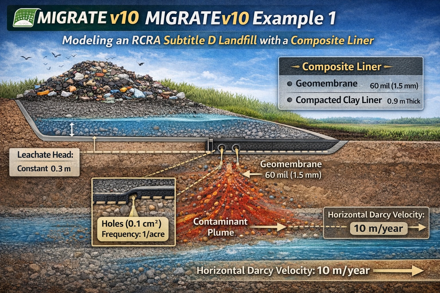
MIGRATEv10 Example 1: Modeling a RCRA Subtitle D Landfill with a Composite Liner
Landfill SystemsComposite liner

Example 1: Modeling a RCRA Subtitle D Landfill with a Composite Liner

Models a composite geomembrane and clay liner, primary leachate collection and aquifer impact.

Open documented example


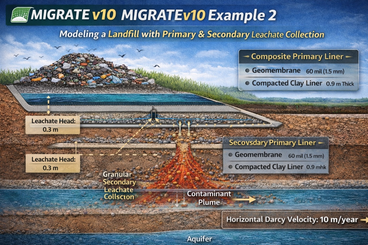
MIGRATEv10 Example 2: Composite Liner System with Primary & Secondary Leachate Collection
Landfill SystemsDual collection

Example 2: Composite Liner System with Primary & Secondary Leachate Collection

Evaluates a multi-barrier landfill with primary and secondary collection systems above an aquitard and aquifer.

Open documented example
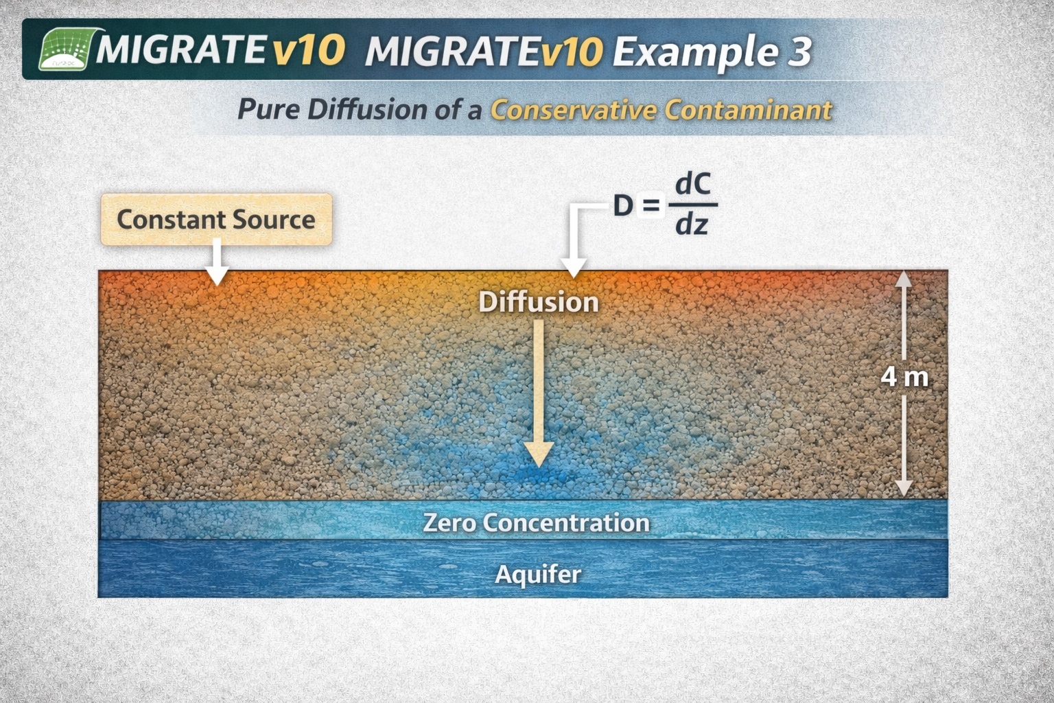
MIGRATEv10 Example 3: Pure Diffusion of a Conservative Contaminant
FundamentalsPure diffusion

Example 3: Pure Diffusion of a Conservative Contaminant

Isolates two-dimensional diffusion without advection or sorption using a zero-concentration lower boundary.

Open documented example
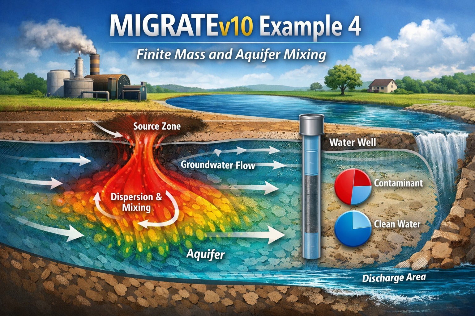
MIGRATEv10 Example 4: Finite Mass Source and Aquifer Mixing with Base Outflow
FundamentalsFinite source

Example 4: Finite Mass Source and Aquifer Mixing with Base Outflow

Combines a depleting source with aquifer mixing and contaminant outflow at the base of the model.

Open documented example
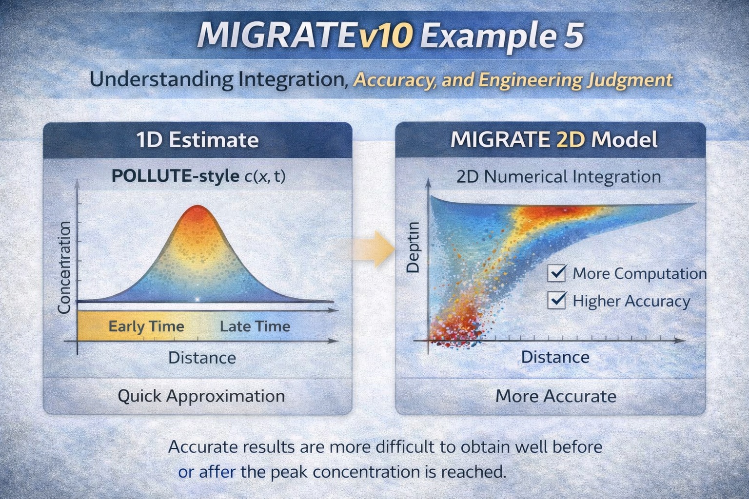
MIGRATEv10 Example 5: Understanding Integration, Accuracy, and the Role of Engineering Judgment
Numerical VerificationEngineering judgment

Example 5: Understanding Integration, Accuracy, and the Role of Engineering Judgment

Explains integration accuracy, dimensional assumptions and the interpretation of preliminary modeling results.

Open documented example
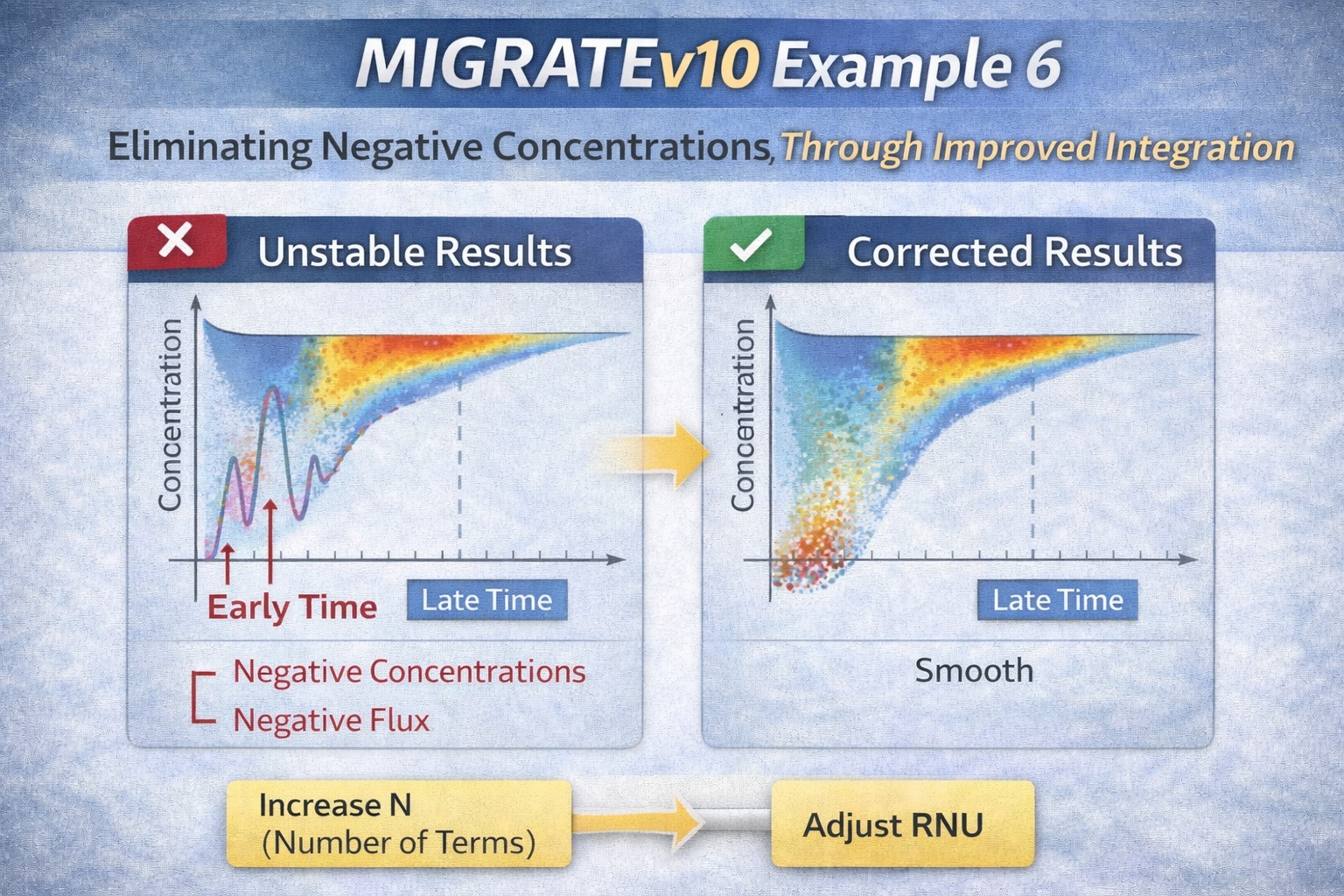
MIGRATEv10 Example 6: Eliminating Negative Concentrations Through Improved Integration
Numerical VerificationTalbot integration

Example 6: Eliminating Negative Concentrations Through Improved Integration

Demonstrates how refined Talbot integration parameters remove numerical artifacts and improve stability.

Open documented example
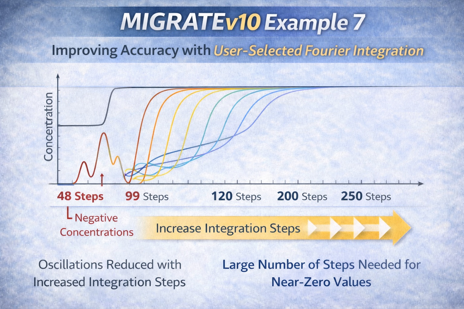
MIGRATEv10 Example 7: Improving Accuracy with User-Selected Fourier Integration
Numerical VerificationFourier integration

Example 7: Improving Accuracy with User-Selected Fourier Integration

Uses user-selected Fourier and Gauss integration controls to reduce oscillation and negative results.

Open documented example
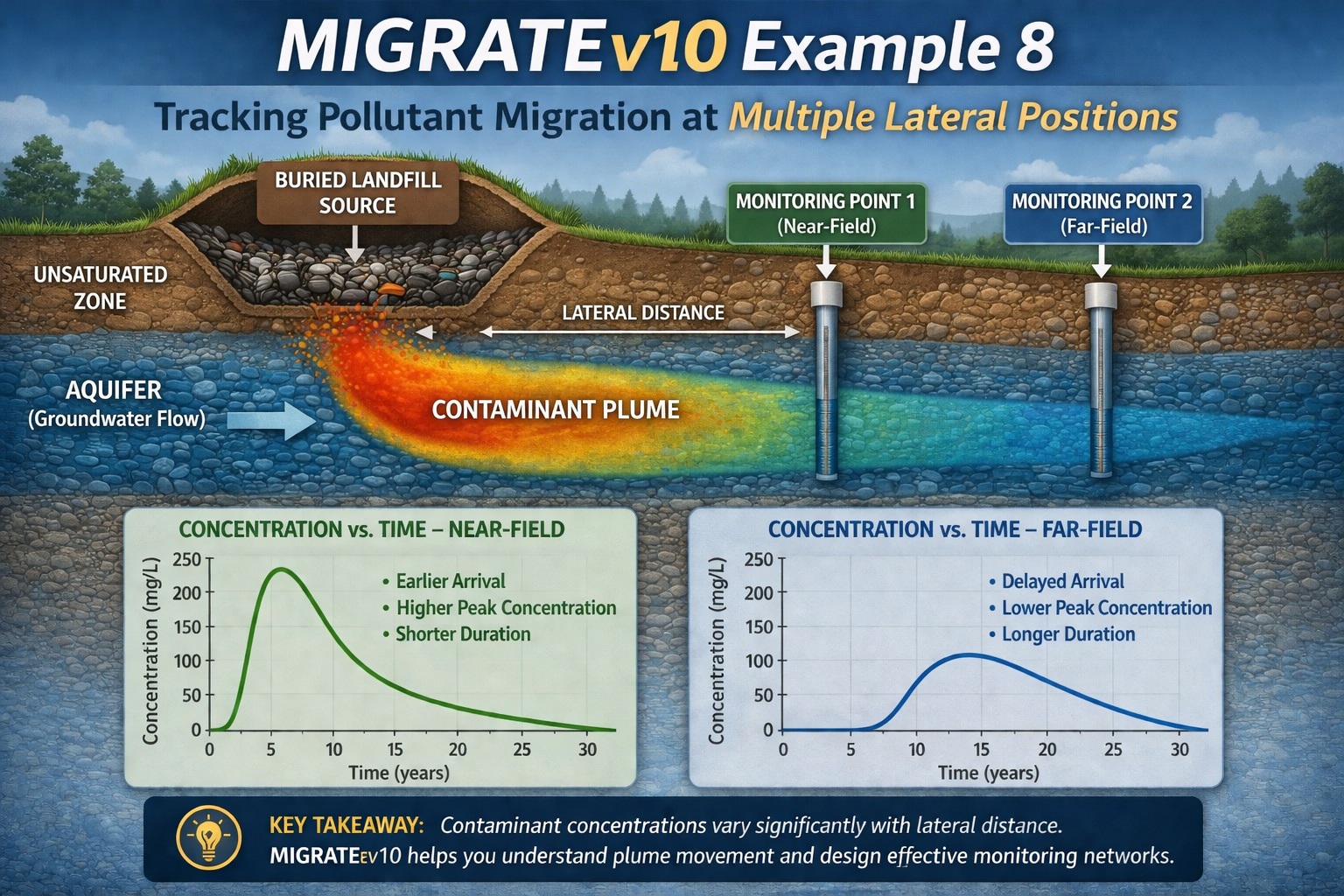
MIGRATEv10 Example 8: Evaluating Contaminant Migration at Multiple Lateral Positions
Spatial & Multi-SourceLateral migration

Example 8: Evaluating Contaminant Migration at Multiple Lateral Positions

Compares concentrations at several lateral positions to reveal two-dimensional plume development.

Open documented example
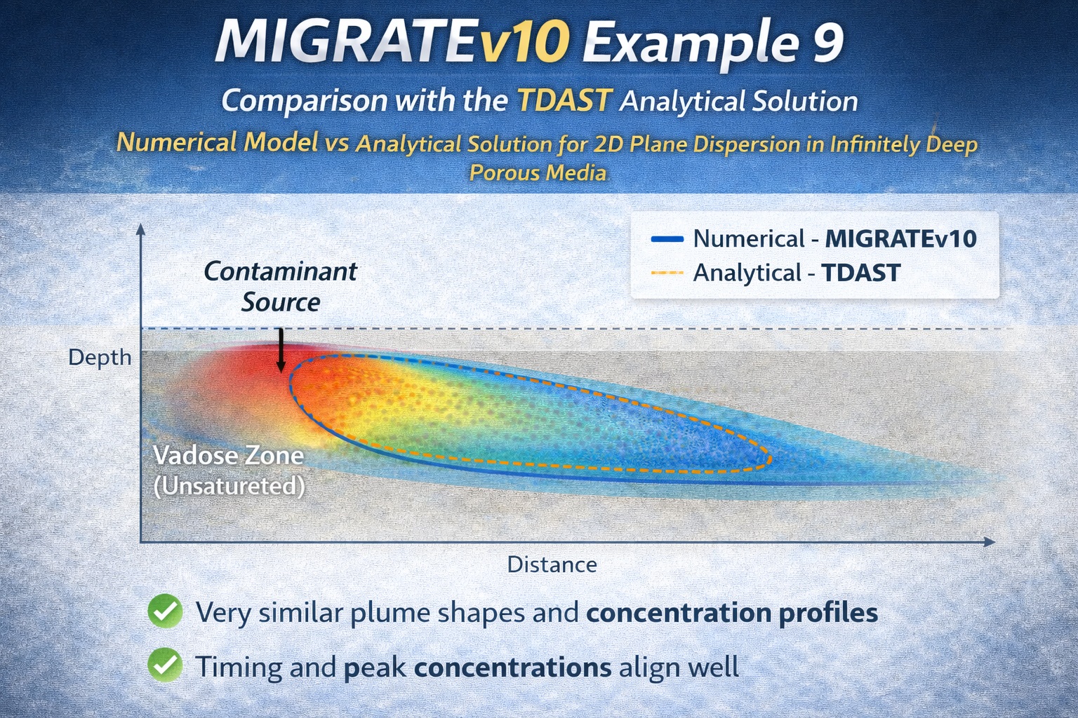
MIGRATEv10 Example 9: Comparison with the TDAST Analytical Solution
Numerical VerificationAnalytical benchmark

Example 9: Comparison with the TDAST Analytical Solution

Benchmarks MIGRATEv10 against the TDAST analytical solution for two-dimensional plane dispersion.

Open documented example
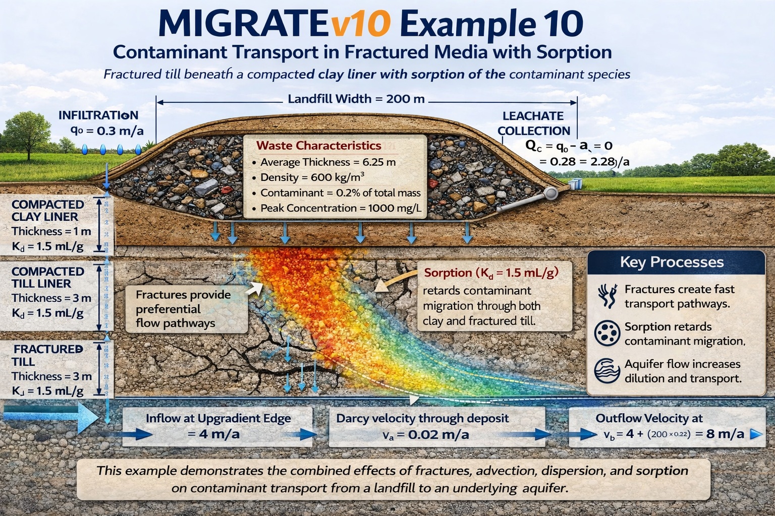
MIGRATEv10 Example 10: Contaminant Transport in Fractured Media with Sorption
Spatial & Multi-SourceFractured media

Example 10: Contaminant Transport in Fractured Media with Sorption

Models two-dimensional transport through fractured till beneath a clay liner with reactive sorption.

Open documented example
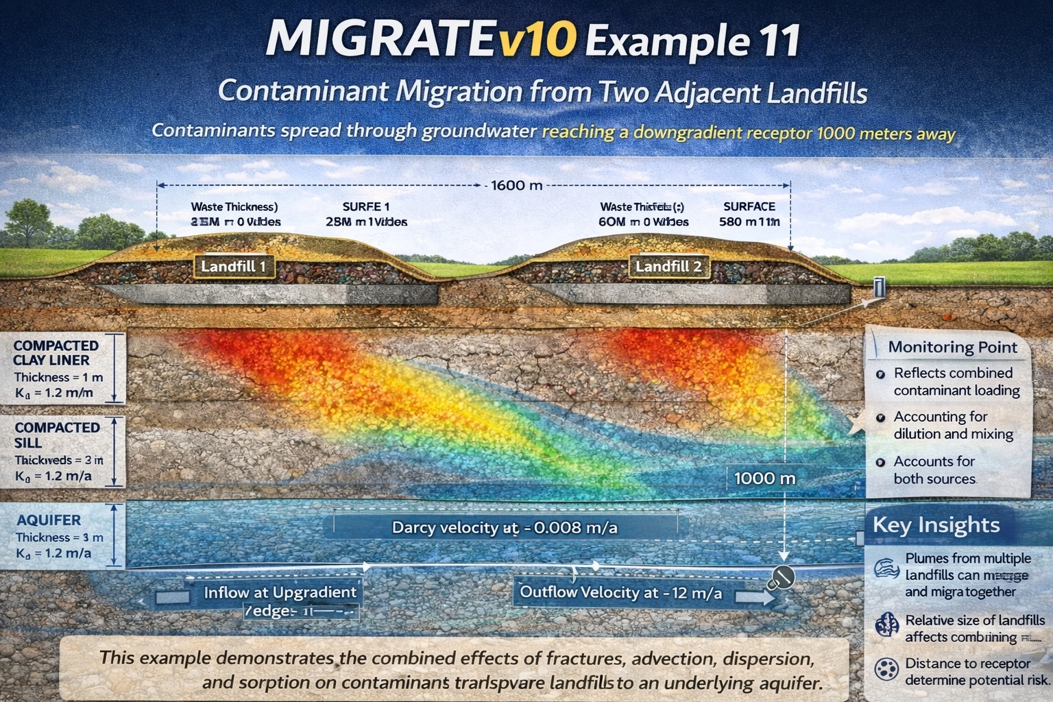
MIGRATEv10 Example 11: Contaminant Migration from Two Adjacent Landfill Cells
Spatial & Multi-SourceMultiple sources

Example 11: Contaminant Migration from Two Adjacent Landfill Cells

Examines interacting plumes from adjacent cells and predicted concentrations at a downgradient receptor.

Open documented example
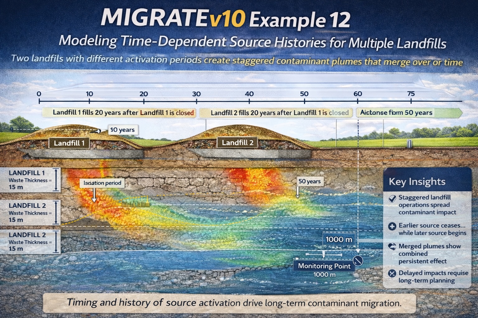
MIGRATEv10 Example 12: Modeling Time-Dependent Source Histories for Multiple Landfill Cells
Spatial & Multi-SourceChanging sources

Example 12: Modeling Time-Dependent Source Histories for Multiple Landfill Cells

Combines multiple landfill cells with distinct time-dependent source histories in one spatial model.

Open documented example
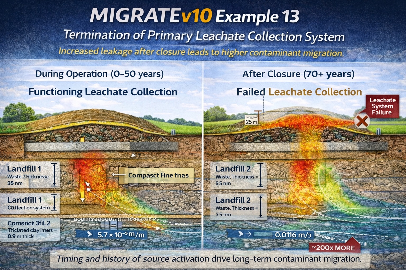
MIGRATEv10 Example 13: Termination of Primary Leachate Collection System
Landfill SystemsSystem termination

Example 13: Termination of Primary Leachate Collection System

Models post-closure collection-system termination using time-dependent leachate head and Darcy velocity.

Open documented example
Instructional examples are not design standards. Adapt the conceptual model and parameters to site-specific conditions and have the resulting engineering interpretation reviewed by a qualified professional.
Suggested Learning Path

Build 2D Modeling Confidence in Four Stages

1

Transport Foundations

Begin with Examples 3 and 4 to understand pure diffusion, finite source mass, aquifer mixing and base outflow.

2

Engineered Landfills

Use Examples 1, 2 and 13 for composite liners, dual collection systems and post-closure termination.

3

Numerical Confidence

Review Examples 5, 6, 7 and 9 for integration controls, artifacts and analytical comparison.

4

Spatial Complexity

Progress through Examples 8, 10, 11 and 12 for lateral, fractured and multi-source transport.

Selecting a Starting Point

Match the Example to the Spatial Question

  • Identify the source geometry, lateral extent and number of sources
  • Determine whether both vertical and lateral concentration gradients matter
  • Choose the required liner, collection, aquitard and aquifer boundaries
  • Identify finite mass, time histories, sorption or fractured-media processes
  • Review integration settings if concentrations oscillate or become negative
  • Use POLLUTEv10 when a simpler layered 1D/1.5D formulation is adequate

Recommended Use of an Example

  1. Reproduce the documented case.
  2. Check its spatial trends and mass behavior.
  3. Save an unchanged reference copy.
  4. Replace inputs with project-supported values.
  5. Test one geometry or parameter change at a time.
  6. Document assumptions, controls and limitations.
Continue Learning

Connect Examples to Product Guidance

MIGRATEv10 Core Features

Review 2D model geometry, lateral positions, multiple sources and output capabilities.

Explore Core Features

POLLUTEv10 Examples

Explore progressive 1D/1.5D cases when full two-dimensional geometry is not required.

Browse POLLUTE Examples

Complete Knowledge Center Archive

Browse the original MIGRATE articles and related contaminant-modeling guidance.

Open the archive

POLLUTE and MIGRATE

Compare the 1D/1.5D and 2D approaches for the project question.

Compare the products

Upgrade Guidance

Plan migration from POLLUTE v7 or MIGRATE v9.

Review Upgrades

Technical Support

Ask about model configuration, installation or product evaluation.

Contact Technical Support

Ready to Reproduce an Example in MIGRATEv10?

Start with the closest documented spatial case, verify its behavior and then introduce project-specific assumptions.